RNNs
NLP Terms
NLP = Natural Language Processing
Embedding
In a general sense, “embedding” refers to the process of representing one kind of object or data in another space or format. It involves mapping objects from a higher-dimensional space into a lower-dimensional space while preserving certain relationships or properties.
— GPT 3.5
For example, the Principal Component Analysis (PCA) algorithm is an embedding technique. PCA is a widely used dimensionality reduction technique that projects high-dimensional data into a lower-dimensional space, while retaining as much of the data’s variance as possible. In my understanding, the constraint on variance in PCA is intended to allow us to distinguish each point as effectively as possible in the new lower-dimensional space. And that is the “preserved property” in this case.
In NLP, the embedding layer is used to obtain the feature vector for each token in the input sequence. One-hot is a simple example of the embedding.
My understanding
Embedding is used for the reality calibration of networks. Essentially, it is a form of semantic alignment. From the perspective of computer science, embedding can be understood as a type of compiler, while from the perspective of data science, it is a simple encoder. However, the design of a compiler relies on various analyses, whereas from the data science viewpoint, it involves optimizing to change the parameters to their optimal target.
The input is something you can understand, and then you want the machine to understand your input and execute related commands. If you imagine it in terms of circuits, it’s like you’re holding a switch, and behind the switch, there are many complex circuits. Then, you know the relationship between your switch and the function you want to achieve, such as designing the circuit so that flipping the switch up means “on” and down means “off.” This whole setup then becomes a form of embedding.
Items $\to$ one-hot variables:
1
2
3
4
5
6
7
8
9
10
11
12
13
14
15
16
17
import torch
import torch.nn.functional as F

A = torch.tensor([3, 0, 2])
output1 = F.one_hot(A)
'''
tensor([[0, 0, 0, 1],
        [1, 0, 0, 0],
        [0, 0, 1, 0]])
'''

output2 = F.one_hot(A, num_classes=5)
'''
tensor([[0, 0, 0, 1, 0],
        [1, 0, 0, 0, 0],
        [0, 0, 1, 0, 0]])
'''
Items $\to$ learnable embedded variables:
1
2
3
4
5
6
7
8
9
10
11
12
13
14
15
16
17
18
19
20
21
22
23
24
25
import torch

torch.manual_seed(1)

words = ["hello", "world", "haha"]
vocab_size = len(words)
idx = list(range(vocab_size))
dictionary = dict(zip(words, idx))  # {'hello': 0, 'world': 1, 'haha': 2}
embedding_dim = 2

embedding_layer = torch.nn.Embedding(num_embeddings=vocab_size,     # how many values in a dim (input)
                                     embedding_dim=embedding_dim)   # output_dim
print(list(embedding_layer.parameters()))
'''
[Parameter containing:
tensor([[ 0.6614,  0.2669],
        [ 0.0617,  0.6213],
        [-0.4519, -0.1661]], requires_grad=True)]
'''

lookup_tensor = torch.tensor([dictionary["haha"]], dtype=torch.long)
haha_embed = embedding_layer(lookup_tensor)
print(haha_embed)
# tensor([[-0.4519, -0.1661]], grad_fn=<EmbeddingBackward0>)
# The result is exactly the third row of the embedding layer parameter matrix.
- Each element in the weight matrix is sampled from $\mathcal{N}(0,1)$.
- “An Embedding layer is essentially just a Linear layer.” (From this website.)
- The
padding_idxparameter: (int, optional) - If specified, the entries at padding_idx do not contribute to the gradient. PAD_TOKEN,<BOS>and others should be considered in thenum_embeddingscount.
Map back:
- Given an embedding result $y$, find the corresponding word $x$.
- Calculate the embeddings of all words $(y_1, \ldots, y_n)$,
- $x = \arg\min_i \Vert y - y_i \Vert$
1
2
3
4
5
6
7

all_embeddings = embedding_layer(torch.arange(vocab_size))
distances = torch.norm(all_embeddings - hello_embed, dim=1)
min_index = torch.argmin(distances).item()
closest_word = [word for word, idx in dictionary.items() if idx == min_index][0]
print(f"Closest word for the given vector: {closest_word}")
# Closest word for the given vector: haha
Integer (index) tensors $\to$ learnable embedded variables:
1
2
3
4
5
6
7
8
9
10
11
12
13
14
15
16
17
18
19
20
21
22
23
24
25
26
27
28
29
30
31
32
33
34
35
36
37
import torch

vocab_size = 10
embedding_dim = 3

embedding_layer = torch.nn.Embedding(vocab_size, embedding_dim)
print(list(embedding_layer.parameters()))
'''
tensor([[-2.3097,  2.8327,  0.2768],
        [-1.8660, -0.5876, -0.5116],
        [-0.6474,  0.7756, -0.1920],
        [-1.2533, -0.7186,  1.8712],
        [-1.5365, -1.0957, -0.9209],
        [-0.0757,  2.3399,  0.9409],
        [-0.9143,  1.3293,  0.8625],
        [ 1.3818, -0.1664, -0.5298],
        [ 2.2011, -0.8805,  1.7162],
        [-0.9934,  0.3914,  0.9149]], requires_grad=True)]
'''

# A batch of 2 samples of 4 indices each
# Each index is in [0, vocab_size - 1]
input = torch.LongTensor([[1, 2, 4, 5],     # Sentence A
                          [4, 3, 2, 9]])    # Sentence B
output = embedding_layer(input)
print(output)
'''
tensor([[[-1.8660, -0.5876, -0.5116],
         [-0.6474,  0.7756, -0.1920],
         [-1.5365, -1.0957, -0.9209],
         [-0.0757,  2.3399,  0.9409]],

        [[-1.5365, -1.0957, -0.9209],
         [-1.2533, -0.7186,  1.8712],
         [-0.6474,  0.7756, -0.1920],
         [-0.9934,  0.3914,  0.9149]]], grad_fn=<EmbeddingBackward0>)
'''
Differentiable embedding
“An Embedding layer is essentially just a Linear layer.” From this website.
1
2
3
embedding_layer = torch.nn.Sequential(
    torch.nn.Linear(input_dim, output_dim, bias=False),
)
Tokenization
Check this website.
1
2
3
4
5
6
7
8
9
10
sentence = 'We do not see things as they are, we see them as we are.'

character_tokenization = list(sentence)
# ['W', 'e', ' ', 'd', 'o', ' ', 'n', 'o', 't', ' ', 's', 'e', 'e', ' ', 't', 'h', 'i', 'n', 'g', 's', ' ', 'a', 's', ' ', 't', 'h', 'e', 'y', ' ', 'a', 'r', 'e', ',', ' ', 'w', 'e', ' ', 's', 'e', 'e', ' ', 't', 'h', 'e', 'm', ' ', 'a', 's', ' ', 'w', 'e', ' ', 'a', 'r', 'e', '.']

word_tokenization = sentence.split()
# ['We', 'do', 'not', 'see', 'things', 'as', 'they', 'are,', 'we', 'see', 'them', 'as', 'we', 'are.']

sentence_tokenization = sentence.split(', ')
# ['We do not see things as they are', 'we see them as we are.']
BoW
BOW = Bag of Words
In my understanding, BoW is a step
- to make and clean a word-level tokenization, and
- to count and store the occurrences of each word.
For instance, given the vocabulary
{apple, banana, cherry}:
- Text:
"apple banana apple"- BoW representation:
{2, 1, 0}— ChatGPT-4
Word2Vec
Word2Vec = Word to Vector
Word2Vec is a group of related models that are used to produce word embeddings. Word2Vec takes a large corpus of text as its input and produces a high-dimensional space (typically of several hundred dimensions), with each unique word in the corpus being assigned a corresponding vector in the space.
— ChatGPT-4
In my understanding:
- During training, the process involves presenting a set of words (the context) and predicting the surrounding words.
- The model learns from reading the corpus to understand the context in which each word occurs in the language.
- If a certain word at a particular position in a context appears frequently in the corpus, then when given that context, the model’s output probability for that word should also be high.
CBOW
CBOW = Continuous Bag of Words
The CBOW model predicts the current word based on its context. The objective function to maximize can be expressed as: \(J(\theta) = \frac{1}{T} \sum_{t=1}^{T} \log p(w_t | C_t)\)
Skip-Gram
The Skip-Gram model predicts the context given a word. Its objective function can be expressed as: \(J(\theta) = \frac{1}{T} \sum_{t=1}^{T} \sum_{-c \leq j \leq c, j \neq 0} \log p(w_{t+j} | w_t)\)
Here, $T$ is the total number of words in the training corpus, and $c$ is the size of the context.
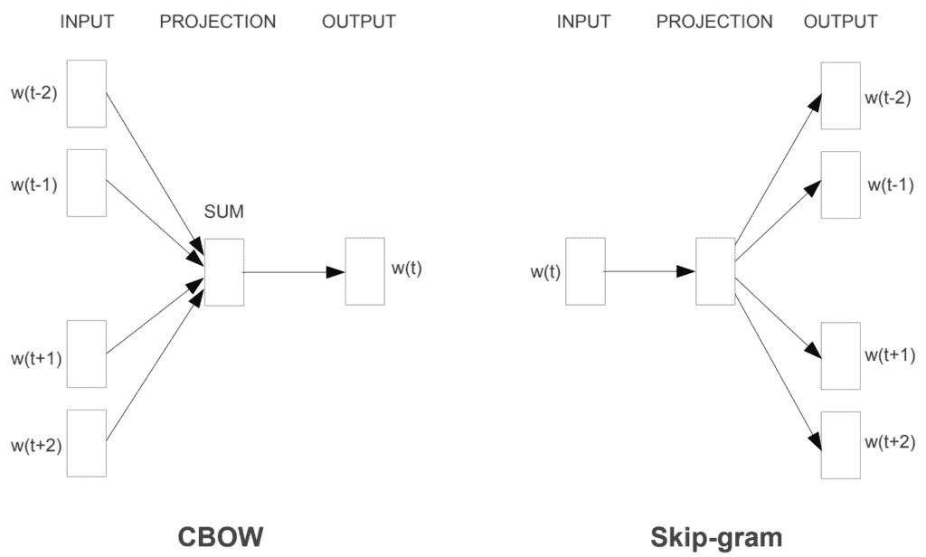 Illustration of CBOW and Skip-Gram from the paper “Exploiting Similarities among Languages for Machine Translation”.
RNN Models
RNN
RNN = Recurrent Neural Network
\[\begin{aligned} \begin{cases} h_t = f_{w_h}(x_t, h_{t-1}) \\ o_t = g_{w_o}(h_t) \\ \end{cases} \end{aligned}\] Illustration of RNN from the book “Dive into Deep Learning”. Boxes represent variables (not shaded) or parameters (shaded) and circles represent operators.
If there are $L$ RNN layers, then
\[\begin{aligned} \begin{cases} h_t^1 = \mathrm{Sigmoid}\left(\mathrm{Linear}(x_t) + \mathrm{Linear}(h_{t-1}^1)\right) \\ h_t^2 = \mathrm{Sigmoid}\left(\mathrm{Linear}(h_t^1) + \mathrm{Linear}(h_{t-1}^2)\right) \\ \ldots \\ o_t = \mathrm{Linear}(h_t^L) \end{cases} \end{aligned}\]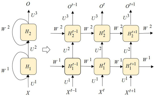 Illustration of Stacked RNN from the paper “RNNCon: Contribution Coverage Testing for Stacked Recurrent Neural Networks”.
1
2
3
4
5
6
7
8
9
10
11
12
13
14
# Adapted from https://pytorch.org/docs/stable/generated/torch.nn.RNN.html
import torch

rnn = torch.nn.RNN(10, 20, 2)   # input_size, hidden_size, num_layers
input = torch.randn(5, 3, 10)   # sequence_length, batch_size, input_size
h0 = torch.randn(2, 3, 20)      # num_layers, batch_size, hidden_size
output, hn = rnn(input, h0)     # h0: Defaults to zeros if not provided.

print(output.size(), hn.size())
# torch.Size([5, 3, 20]) torch.Size([2, 3, 20])
# output size: sequence_length, batch_size, hidden_size

# If parameter batch_first=True,
# then the first parameter should be the batch_size.
In NLP:
- An input is a sentence. The
sequence_lengthis the number of words in the sentence. - The
input_sizeis the embedding dimension of each word. - The
output_sizeequals thesequence_length. - All the hidden states have the same
hidden_size.
An example that makes it easy to remember the dimensions of various quantities:
1
2
3
4
5
6
7
8
9
10
11
12
13
14
15
16
17
18
19
20
21
22
23
24
25
26
27
28
29
30
# input_size = embedding_dim = 3
embedded_words = {"I": [0.3, 0.5, 0.1],
                  "am": [0.4, 0.4, 0.3],
                  "so": [0.1, 0.9, 0.2],
                  "happy": [0.5, 0.3, 0.8],
                  "sad": [0.2, 0.6, 0.1],
                  ".": [0.6, 0.2, 0.6],
                  "<EOS>": [0.0, 0.0, 0.0],
                  "<PAD>": [0.9, 0.9, 0.9]}

sentences = ["I am so happy.",
             "I am sad."]

# dataset_size = (batch_size, sequence_length, embedding_dim) = (2, 6, 3,)
# sequence_length = max(sentence_length); Padding
embedded_sentences = [[[0.3, 0.5, 0.1],
                       [0.4, 0.4, 0.3],
                       [0.1, 0.9, 0.2],
                       [0.5, 0.3, 0.8],
                       [0.2, 0.6, 0.1],
                       [0.0, 0.0, 0.0]],

                      [[0.3, 0.5, 0.1],
                       [0.4, 0.4, 0.3],
                       [0.5, 0.3, 0.8],
                       [0.6, 0.2, 0.6],
                       [0.0, 0.0, 0.0],
                       [0.9, 0.9, 0.9]]]

# hidden_size, num_layers: determined by parameter tuning :)
BPTT
BPTT = Backpropagation Through Time
\(L = \frac{1}{T}\sum\limits_{t} l(o_t,y_t)\) \(\begin{aligned} \frac{\partial L}{\partial w_o} =& \frac{1}{T}\sum\limits_{t} \frac{\partial l(y_t,o_t)}{\partial w_o} \\ =& \frac{1}{T}\sum\limits_{t} \frac{\partial l(y_t,o_t)}{\partial o_t}\cdot \frac{\partial o_t}{\partial w_o} \end{aligned}\) \(\begin{aligned} \frac{\partial L}{\partial w_h} =& \frac{1}{T}\sum\limits_{t} \frac{\partial l(y_t,o_t)}{\partial w_h} \\ =& \frac{1}{T}\sum\limits_{t} \frac{\partial l(y_t,o_t)}{\partial o_t} \cdot \frac{\partial o_t}{\partial h_t} \cdot \textcolor{red}{\frac{\partial h_t}{\partial w_h}} \end{aligned}\)
\[\begin{aligned} \textcolor{red}{\frac{\partial h_t}{\partial w_h}} =& \frac{\partial f(x_t, h_{t-1}, w_h)}{\partial w_h} + \frac{\partial f(x_t, h_{t-1}, w_h)}{\partial h_{t-1}} \cdot \textcolor{red}{\frac{\partial h_{t-1}}{\partial w_h}} \end{aligned}\] \[\begin{cases} z_0 = a_0 = 0 \\ z_k = a_k + b_k \cdot z_{k-1} \\ \end{cases}\] \[\begin{aligned} z_k = a_k + \sum\limits_{i=0}^{k-1} \left(\prod\limits_{j=i+1}^k b_j \right) \cdot a_i \end{aligned}\]LSTM
LSTM = Long Short-Term Memory
- To learn long-term dependencies (owing to vanishing and exploding gradients).
- In my understanding, there are two kinds of hidden states, $\mathrm{c}$ and $\mathrm{h}$. And $\mathrm{c}$ is renamed as the memory cell internal state.
Each layer is like:
\[\begin{aligned} \begin{cases} i_t =& \mathrm{Sigmoid}\left(\mathrm{Linear}(x_t) + \mathrm{Linear}(h_{t-1})\right) \\ f_t =& \mathrm{Sigmoid}\left(\mathrm{Linear}(x_t) + \mathrm{Linear}(h_{t-1})\right) \\ g_t =& \mathrm{tanh}\left(\mathrm{Linear}(x_t) + \mathrm{Linear}(h_{t-1})\right) \\ o_t =& \mathrm{Sigmoid}\left(\mathrm{Linear}(x_t) + \mathrm{Linear}(h_{t-1})\right) \\ c_t =& f_t \odot c_{t-1} + i_t \odot g_t \\ h_t =& o_t \odot \mathrm{tanh}(c_t) \end{cases} \end{aligned}\]Adapted from the PyTorch document.
- $h_t$: the hidden state.
- $c_t$: the cell state.
- $i_t$: the input gate.
- $f_t$: the forget gate.
- $g_t$: the cell gate.
- $o_t$: the output gate.
- All values of the three gates are in the range of $(0, 1)$ because of the sigmoid function.
- $g_t$ is the vanilla part of an RNN, and it indicates the information that we currently get.
- $i_t$ controls how much we cares about the current information.
- $c$ is an addtional hidden state channel, and it also indicates the memory.
- $f_t$ controls how much we cares about the memory.
- $c_t$ and $h_t$ do not impact the curren output $o_t$.
 Illustration of LSTM from the book “Dive into Deep Learning”.
1
2
3
4
5
6
7
8
9
10
11
12
13
14
15
# Adapted from https://pytorch.org/docs/stable/generated/torch.nn.LSTM.html
import torch

rnn = torch.nn.LSTM(10, 20, 2)    # input_size, hidden_size, num_layers
input = torch.randn(5, 3, 10)     # sequence_length, batch_size, input_size
h0 = torch.randn(2, 3, 20)        # num_layers, batch_size, hidden_size
c0 = torch.randn(2, 3, 20)        # num_layers, batch_size, hidden_size
output, (hn, cn) = rnn(input, (h0, c0)) # h0: Defaults to zeros if not provided.

print(output.size(), hn.size(), cn.size())
# torch.Size([5, 3, 20]) torch.Size([2, 3, 20]) torch.Size([2, 3, 20])
# output size: sequence_length, batch_size, hidden_size

# If parameter batch_first=True,
# then the first parameter should be the batch_size.
GRU
GRU = Gated Recurrent Units
Each layer is like:
\[\begin{aligned} \begin{cases} r_t =& \mathrm{Sigmoid}\left(\mathrm{Linear}(x_t) + \mathrm{Linear}(h_{t-1})\right) \\ z_t =& \mathrm{Sigmoid}\left(\mathrm{Linear}(x_t) + \mathrm{Linear}(h_{t-1})\right) \\ n_t =& \mathrm{tanh}\left(\mathrm{Linear}(x_t) + r_t \odot \mathrm{Linear}(h_{t-1})\right) \\ h_t =& (1-z_t)\odot n_t + z \odot h_{t-1} \end{cases} \end{aligned}\]- $h_t$: the hidden state. It can be used as the output.
- $r_t$: the reset gate, controls how much we cares about the memory. It is a bit like the forget gate $f_t$ in LSTM
- $z_t$: the update gate, controls how much we cares about the current information. It is a bit like the input gate $i_t$ in LSTM.
- $n_t$: the candidate hidden state, or the new gate.
- If the reset gate $r_t$ is close to $1$, then it is like the vanilla RNN.
- If the reset gate $r_t$ is close to $0$, then the new gate $n_t$ is the result of an MLP of $x_t$.
 Illustration of GRU from the book “Dive into Deep Learning”.
1
2
3
4
5
6
7
8
9
10
11
12
13
14
15
16
17
# Adapted from https://pytorch.org/docs/stable/generated/torch.nn.GRU.html
import torch

rnn = torch.nn.GRU(10, 20, 2)   # input_size, hidden_size, num_layers
input = torch.randn(5, 3, 10)   # sequence_length, batch_size, input_size
h0 = torch.randn(2, 3, 20)      # num_layers, batch_size, hidden_size
output, hn = rnn(input, h0)     # h0: Defaults to zeros if not provided.

print(output.size(), hn.size())
# torch.Size([5, 3, 20]) torch.Size([2, 3, 20])
# output size: sequence_length, batch_size, hidden_size

# If parameter batch_first=True,
# then the first parameter should be the batch_size.

are_close = torch.allclose(output, hn, atol=1e-3)
print(are_close)
1
2
3
4
Traceback (most recent call last):
  File "/Users/luna/Documents/RL/project/9_CompactMARL/my_test/gru_test.py", line 12, in <module>
    are_close = torch.allclose(output, hn, atol=1e-3)
RuntimeError: The size of tensor a (5) must match the size of tensor b (2) at non-singleton dimension 0
1
2
3
4
5
6
7
8
9
10
11
12
13
import torch

rnn = torch.nn.GRU(10, 20, 2)   # input_size, hidden_size, num_layers
input = torch.randn(5, 3, 10)   # sequence_length, batch_size, input_size
h0 = torch.randn(2, 3, 20)      # num_layers, batch_size, hidden_size
output, hn = rnn(input, h0)     # h0: Defaults to zeros if not provided.

print(output.size(), hn.size())
# torch.Size([5, 3, 20]) torch.Size([2, 3, 20])
# output size: sequence_length, batch_size, hidden_size

last_are_close = torch.allclose(output[-1], hn[-1], atol=1e-3)
print(last_are_close)
1
2
torch.Size([5, 3, 20]) torch.Size([2, 3, 20])
True