Sequence-to-Sequence Models

NLP Terms

NLP = Natural Language Processing

Embedding

In a general sense, “embedding” refers to the process of representing one kind of object or data in another space or format. It involves mapping objects from a higher-dimensional space into a lower-dimensional space while preserving certain relationships or properties.

— GPT 3.5

For example, the Principal Component Analysis (PCA) algorithm is an embedding technique. PCA is a widely used dimensionality reduction technique that projects high-dimensional data into a lower-dimensional space, while retaining as much of the data’s variance as possible. In my understanding, the constraint on variance in PCA is intended to allow us to distinguish each point as effectively as possible in the new lower-dimensional space. And that is the “preserved property” in this case.

In NLP, the embedding layer is used to obtain the feature vector for each token in the input sequence. One-hot is a simple example of the embedding.

My understanding

Embedding is used for the reality calibration of networks. Essentially, it is a form of semantic alignment. From the perspective of computer science, embedding can be understood as a type of compiler, while from the perspective of data science, it is a simple encoder. However, the design of a compiler relies on various analyses, whereas from the data science viewpoint, it involves optimizing to change the parameters to their optimal target.

The input is something you can understand, and then you want the machine to understand your input and execute related commands. If you imagine it in terms of circuits, it’s like you’re holding a switch, and behind the switch, there are many complex circuits. Then, you know the relationship between your switch and the function you want to achieve, such as designing the circuit so that flipping the switch up means “on” and down means “off.” This whole setup then becomes a form of embedding.

Items $\to$ one-hot variables:

import torch
import torch.nn.functional as F

A = torch.tensor([3, 0, 2])
output1 = F.one_hot(A)
'''
tensor([[0, 0, 0, 1],
        [1, 0, 0, 0],
        [0, 0, 1, 0]])
'''

output2 = F.one_hot(A, num_classes=5)
'''
tensor([[0, 0, 0, 1, 0],
        [1, 0, 0, 0, 0],
        [0, 0, 1, 0, 0]])
'''

Items $\to$ learnable embedded variables:

import torch

torch.manual_seed(1)

words = ["hello", "world", "haha"]
vocab_size = len(words)
idx = list(range(vocab_size))
dictionary = dict(zip(words, idx))  # {'hello': 0, 'world': 1, 'haha': 2}
embedding_dim = 2

embedding_layer = torch.nn.Embedding(num_embeddings=vocab_size,     # how many values in a dim (input)
                                     embedding_dim=embedding_dim)   # output_dim
print(list(embedding_layer.parameters()))
'''
[Parameter containing:
tensor([[ 0.6614,  0.2669],
        [ 0.0617,  0.6213],
        [-0.4519, -0.1661]], requires_grad=True)]
'''

lookup_tensor = torch.tensor([dictionary["haha"]], dtype=torch.long)
haha_embed = embedding_layer(lookup_tensor)
print(haha_embed)
# tensor([[-0.4519, -0.1661]], grad_fn=<EmbeddingBackward0>)
# The result is exactly the third row of the embedding layer parameter matrix.

torch.nn.Embedding:

• Each element in the weight matrix is sampled from $\mathcal{N}(0,1)$.
• “An Embedding layer is essentially just a Linear layer.” (From this website.)
• The padding_idx parameter: (int, optional) - If specified, the entries at padding_idx do not contribute to the gradient.
• PAD_TOKEN, <BOS> and others should be considered in the num_embeddings count.

Map back:

• Given an embedding result $y$, find the corresponding word $x$.
• Calculate the embeddings of all words $(y_1, \ldots, y_n)$,
• $x = \arg\min_i \Vert y - y_i \Vert$

all_embeddings = embedding_layer(torch.arange(vocab_size))
distances = torch.norm(all_embeddings - hello_embed, dim=1)
min_index = torch.argmin(distances).item()
closest_word = [word for word, idx in dictionary.items() if idx == min_index][0]
print(f"Closest word for the given vector: {closest_word}")
# Closest word for the given vector: haha

Integer (index) tensors $\to$ learnable embedded variables:

import torch

vocab_size = 10
embedding_dim = 3

embedding_layer = torch.nn.Embedding(vocab_size, embedding_dim)
print(list(embedding_layer.parameters()))
'''
tensor([[-2.3097,  2.8327,  0.2768],
        [-1.8660, -0.5876, -0.5116],
        [-0.6474,  0.7756, -0.1920],
        [-1.2533, -0.7186,  1.8712],
        [-1.5365, -1.0957, -0.9209],
        [-0.0757,  2.3399,  0.9409],
        [-0.9143,  1.3293,  0.8625],
        [ 1.3818, -0.1664, -0.5298],
        [ 2.2011, -0.8805,  1.7162],
        [-0.9934,  0.3914,  0.9149]], requires_grad=True)]
'''

# A batch of 2 samples of 4 indices each
# Each index is in [0, vocab_size - 1]
input = torch.LongTensor([[1, 2, 4, 5],     # Sentence A
                          [4, 3, 2, 9]])    # Sentence B
output = embedding_layer(input)
print(output)
'''
tensor([[[-1.8660, -0.5876, -0.5116],
         [-0.6474,  0.7756, -0.1920],
         [-1.5365, -1.0957, -0.9209],
         [-0.0757,  2.3399,  0.9409]],

        [[-1.5365, -1.0957, -0.9209],
         [-1.2533, -0.7186,  1.8712],
         [-0.6474,  0.7756, -0.1920],
         [-0.9934,  0.3914,  0.9149]]], grad_fn=<EmbeddingBackward0>)
'''

Differentiable embedding

“An Embedding layer is essentially just a Linear layer.” From this website.

embedding_layer = torch.nn.Sequential(
    torch.nn.Linear(input_dim, output_dim, bias=False),
)

Tokenization

Check this website.

sentence = 'We do not see things as they are, we see them as we are.'

character_tokenization = list(sentence)
# ['W', 'e', ' ', 'd', 'o', ' ', 'n', 'o', 't', ' ', 's', 'e', 'e', ' ', 't', 'h', 'i', 'n', 'g', 's', ' ', 'a', 's', ' ', 't', 'h', 'e', 'y', ' ', 'a', 'r', 'e', ',', ' ', 'w', 'e', ' ', 's', 'e', 'e', ' ', 't', 'h', 'e', 'm', ' ', 'a', 's', ' ', 'w', 'e', ' ', 'a', 'r', 'e', '.']

word_tokenization = sentence.split()
# ['We', 'do', 'not', 'see', 'things', 'as', 'they', 'are,', 'we', 'see', 'them', 'as', 'we', 'are.']

sentence_tokenization = sentence.split(', ')
# ['We do not see things as they are', 'we see them as we are.']

BoW

BOW = Bag of Words

In my understanding, BoW is a step

• to make and clean a word-level tokenization, and
• to count and store the occurrences of each word.

For instance, given the vocabulary {apple, banana, cherry}:

• Text: "apple banana apple"
• BoW representation: {2, 1, 0}

— ChatGPT-4

Word2Vec

Word2Vec = Word to Vector

Word2Vec is a group of related models that are used to produce word embeddings. Word2Vec takes a large corpus of text as its input and produces a high-dimensional space (typically of several hundred dimensions), with each unique word in the corpus being assigned a corresponding vector in the space.

— ChatGPT-4

In my understanding:

• During training, the process involves presenting a set of words (the context) and predicting the surrounding words.
• The model learns from reading the corpus to understand the context in which each word occurs in the language.
• If a certain word at a particular position in a context appears frequently in the corpus, then when given that context, the model’s output probability for that word should also be high.

CBOW

CBOW = Continuous Bag of Words

The CBOW model predicts the current word based on its context. The objective function to maximize can be expressed as: \(J(\theta) = \frac{1}{T} \sum_{t=1}^{T} \log p(w_t | C_t)\)

Skip-Gram

The Skip-Gram model predicts the context given a word. Its objective function can be expressed as: \(J(\theta) = \frac{1}{T} \sum_{t=1}^{T} \sum_{-c \leq j \leq c, j \neq 0} \log p(w_{t+j} | w_t)\)

Here, $T$ is the total number of words in the training corpus, and $c$ is the size of the context.

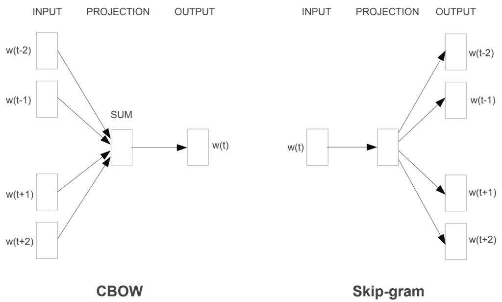Illustration of CBOW and Skip-Gram from the paper “Exploiting Similarities among Languages for Machine Translation”.

RNN Models

RNN

RNN = Recurrent Neural Network

\[\begin{aligned} \begin{cases} h_t = f_{w_h}(x_t, h_{t-1}) \\ o_t = g_{w_o}(h_t) \\ \end{cases} \end{aligned}\]

Illustration of RNN from the book “Dive into Deep Learning”. Boxes represent variables (not shaded) or parameters (shaded) and circles represent operators.

If there are $L$ RNN layers, then

\[\begin{aligned} \begin{cases} h_t^1 = \mathrm{Sigmoid}\left(\mathrm{Linear}(x_t) + \mathrm{Linear}(h_{t-1}^1)\right) \\ h_t^2 = \mathrm{Sigmoid}\left(\mathrm{Linear}(h_t^1) + \mathrm{Linear}(h_{t-1}^2)\right) \\ \ldots \\ o_t = \mathrm{Linear}(h_t^L) \end{cases} \end{aligned}\]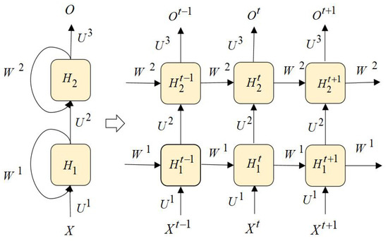

Illustration of Stacked RNN from the paper “RNNCon: Contribution Coverage Testing for Stacked Recurrent Neural Networks”.

# Adapted from https://pytorch.org/docs/stable/generated/torch.nn.RNN.html
import torch

rnn = torch.nn.RNN(10, 20, 2)   # input_size, hidden_size, num_layers
input = torch.randn(5, 3, 10)   # sequence_length, batch_size, input_size
h0 = torch.randn(2, 3, 20)      # num_layers, batch_size, hidden_size
output, hn = rnn(input, h0)     # h0: Defaults to zeros if not provided.

print(output.size(), hn.size())
# torch.Size([5, 3, 20]) torch.Size([2, 3, 20])
# output size: sequence_length, batch_size, hidden_size

# If parameter batch_first=True,
# then the first parameter should be the batch_size.

In NLP:

• An input is a sentence. The sequence_length is the number of words in the sentence.
• The input_size is the embedding dimension of each word.
• The output_size equals the sequence_length.
• All the hidden states have the same hidden_size.

An example that makes it easy to remember the dimensions of various quantities:

# input_size = embedding_dim = 3
embedded_words = {"I": [0.3, 0.5, 0.1],
                  "am": [0.4, 0.4, 0.3],
                  "so": [0.1, 0.9, 0.2],
                  "happy": [0.5, 0.3, 0.8],
                  "sad": [0.2, 0.6, 0.1],
                  ".": [0.6, 0.2, 0.6],
                  "<EOS>": [0.0, 0.0, 0.0],
                  "<PAD>": [0.9, 0.9, 0.9]}

sentences = ["I am so happy.",
             "I am sad."]

# dataset_size = (batch_size, sequence_length, embedding_dim) = (2, 6, 3,)
# sequence_length = max(sentence_length); Padding
embedded_sentences = [[[0.3, 0.5, 0.1],
                       [0.4, 0.4, 0.3],
                       [0.1, 0.9, 0.2],
                       [0.5, 0.3, 0.8],
                       [0.2, 0.6, 0.1],
                       [0.0, 0.0, 0.0]],

                      [[0.3, 0.5, 0.1],
                       [0.4, 0.4, 0.3],
                       [0.5, 0.3, 0.8],
                       [0.6, 0.2, 0.6],
                       [0.0, 0.0, 0.0],
                       [0.9, 0.9, 0.9]]]

# hidden_size, num_layers: determined by parameter tuning :)

BPTT

BPTT = Backpropagation Through Time

\(L = \frac{1}{T}\sum\limits_{t} l(o_t,y_t)\)
\(\begin{aligned} \frac{\partial L}{\partial w_o} =& \frac{1}{T}\sum\limits_{t} \frac{\partial l(y_t,o_t)}{\partial w_o} \\ =& \frac{1}{T}\sum\limits_{t} \frac{\partial l(y_t,o_t)}{\partial o_t}\cdot \frac{\partial o_t}{\partial w_o} \end{aligned}\)
\(\begin{aligned} \frac{\partial L}{\partial w_h} =& \frac{1}{T}\sum\limits_{t} \frac{\partial l(y_t,o_t)}{\partial w_h} \\ =& \frac{1}{T}\sum\limits_{t} \frac{\partial l(y_t,o_t)}{\partial o_t} \cdot \frac{\partial o_t}{\partial h_t} \cdot \textcolor{red}{\frac{\partial h_t}{\partial w_h}} \end{aligned}\)

\[\begin{aligned} \textcolor{red}{\frac{\partial h_t}{\partial w_h}} =& \frac{\partial f(x_t, h_{t-1}, w_h)}{\partial w_h} + \frac{\partial f(x_t, h_{t-1}, w_h)}{\partial h_{t-1}} \cdot \textcolor{red}{\frac{\partial h_{t-1}}{\partial w_h}} \end{aligned}\] \[\begin{cases} z_0 = a_0 = 0 \\ z_k = a_k + b_k \cdot z_{k-1} \\ \end{cases}\] \[\begin{aligned} z_k = a_k + \sum\limits_{i=0}^{k-1} \left(\prod\limits_{j=i+1}^k b_j \right) \cdot a_i \end{aligned}\]

LSTM

LSTM = Long Short-Term Memory

• To learn long-term dependencies (owing to vanishing and exploding gradients).
• In my understanding, there are two kinds of hidden states, $\mathrm{c}$ and $\mathrm{h}$. And $\mathrm{c}$ is renamed as the memory cell internal state.

Each layer is like:

\[\begin{aligned} \begin{cases} i_t =& \mathrm{Sigmoid}\left(\mathrm{Linear}(x_t) + \mathrm{Linear}(h_{t-1})\right) \\ f_t =& \mathrm{Sigmoid}\left(\mathrm{Linear}(x_t) + \mathrm{Linear}(h_{t-1})\right) \\ g_t =& \mathrm{tanh}\left(\mathrm{Linear}(x_t) + \mathrm{Linear}(h_{t-1})\right) \\ o_t =& \mathrm{Sigmoid}\left(\mathrm{Linear}(x_t) + \mathrm{Linear}(h_{t-1})\right) \\ c_t =& f_t \odot c_{t-1} + i_t \odot g_t \\ h_t =& o_t \odot \mathrm{tanh}(c_t) \end{cases} \end{aligned}\]

Adapted from the PyTorch document.

• $h_t$: the hidden state.
• $c_t$: the cell state.
• $i_t$: the input gate.
• $f_t$: the forget gate.
• $g_t$: the cell gate.
• $o_t$: the output gate.
• All values of the three gates are in the range of $(0, 1)$ because of the sigmoid function.
• $g_t$ is the vanilla part of an RNN, and it indicates the information that we currently get.
• $i_t$ controls how much we cares about the current information.
• $c$ is an addtional hidden state channel, and it also indicates the memory.
• $f_t$ controls how much we cares about the memory.
• $c_t$ and $h_t$ do not impact the curren output $o_t$.

Illustration of LSTM from the book “Dive into Deep Learning”.

# Adapted from https://pytorch.org/docs/stable/generated/torch.nn.LSTM.html
import torch

rnn = torch.nn.LSTM(10, 20, 2)    # input_size, hidden_size, num_layers
input = torch.randn(5, 3, 10)     # sequence_length, batch_size, input_size
h0 = torch.randn(2, 3, 20)        # num_layers, batch_size, hidden_size
c0 = torch.randn(2, 3, 20)        # num_layers, batch_size, hidden_size
output, (hn, cn) = rnn(input, (h0, c0)) # h0: Defaults to zeros if not provided.

print(output.size(), hn.size(), cn.size())
# torch.Size([5, 3, 20]) torch.Size([2, 3, 20]) torch.Size([2, 3, 20])
# output size: sequence_length, batch_size, hidden_size

# If parameter batch_first=True,
# then the first parameter should be the batch_size.

GRU

GRU = Gated Recurrent Units

Each layer is like:

\[\begin{aligned} \begin{cases} r_t =& \mathrm{Sigmoid}\left(\mathrm{Linear}(x_t) + \mathrm{Linear}(h_{t-1})\right) \\ z_t =& \mathrm{Sigmoid}\left(\mathrm{Linear}(x_t) + \mathrm{Linear}(h_{t-1})\right) \\ n_t =& \mathrm{tanh}\left(\mathrm{Linear}(x_t) + r_t \odot \mathrm{Linear}(h_{t-1})\right) \\ h_t =& (1-z_t)\odot n_t + z \odot h_{t-1} \end{cases} \end{aligned}\]

• $h_t$: the hidden state. It can be used as the output.
• $r_t$: the reset gate, controls how much we cares about the memory. It is a bit like the forget gate $f_t$ in LSTM
• $z_t$: the update gate, controls how much we cares about the current information. It is a bit like the input gate $i_t$ in LSTM.
• $n_t$: the candidate hidden state, or the new gate.
  • If the reset gate $r_t$ is close to $1$, then it is like the vanilla RNN.
  • If the reset gate $r_t$ is close to $0$, then the new gate $n_t$ is the result of an MLP of $x_t$.

Illustration of GRU from the book “Dive into Deep Learning”.

# Adapted from https://pytorch.org/docs/stable/generated/torch.nn.GRU.html
import torch

rnn = torch.nn.GRU(10, 20, 2)   # input_size, hidden_size, num_layers
input = torch.randn(5, 3, 10)   # sequence_length, batch_size, input_size
h0 = torch.randn(2, 3, 20)      # num_layers, batch_size, hidden_size
output, hn = rnn(input, h0)     # h0: Defaults to zeros if not provided.

print(output.size(), hn.size())
# torch.Size([5, 3, 20]) torch.Size([2, 3, 20])
# output size: sequence_length, batch_size, hidden_size

# If parameter batch_first=True,
# then the first parameter should be the batch_size.

are_close = torch.allclose(output, hn, atol=1e-3)
print(are_close)

Traceback (most recent call last):
  File "/Users/luna/Documents/RL/project/9_CompactMARL/my_test/gru_test.py", line 12, in <module>
    are_close = torch.allclose(output, hn, atol=1e-3)
RuntimeError: The size of tensor a (5) must match the size of tensor b (2) at non-singleton dimension 0

import torch

rnn = torch.nn.GRU(10, 20, 2)   # input_size, hidden_size, num_layers
input = torch.randn(5, 3, 10)   # sequence_length, batch_size, input_size
h0 = torch.randn(2, 3, 20)      # num_layers, batch_size, hidden_size
output, hn = rnn(input, h0)     # h0: Defaults to zeros if not provided.

print(output.size(), hn.size())
# torch.Size([5, 3, 20]) torch.Size([2, 3, 20])
# output size: sequence_length, batch_size, hidden_size

last_are_close = torch.allclose(output[-1], hn[-1], atol=1e-3)
print(last_are_close)

torch.Size([5, 3, 20]) torch.Size([2, 3, 20])
True

---

Encoder-Decoder

Variable-length inputs

• Truncation and Padding
  • Dive Into Deep Learning 10.5.3
• Relation Network
  • A blog
  • ICLR 2017
• Embedding.
• Encoder-decoder.

In general sequence-to-sequence problems like machine translation (Section 10.5), inputs and outputs are of varying lengths that are unaligned. The standard approach to handling this sort of data is to design an encoder–decoder architecture (Fig. 10.6.1) … — Dive into Deep Learning.

The structure

Illustration of the encoder-decoder architecture from the book “Dive into Deep Learning”.

• Encoder: "Hello, world." $\to$ a hidden state (or context variable) of fixed-shape.
• Decoder 1: the state $\to$ "你好，世界。"
• Decoder 2: the state $\to$ "Hola mundo"

Illustration of the encoder-decoder architecture (teacher forcing) from the book “Dive into Deep Learning”.

Illustration of the encoder-decoder architecture (prediction) from the book “Dive into Deep Learning”.

The encoder and the decoder are usually RNNs.

• <eos> means the end of the sequence.
  • Inputting <eos> into the encoder indicates the end of this sentence.
  • In prediction: When the decoder outputs <eos>, it will automatically stop and no longer continue generating output.
• <bos> means the beginning of the sequence, used to signal the decoder when to begin generating a new sequence.
• The input of the encoder is a variable-length sequence, but its output is of fixed-length, named as the state or the context variable $c$.
• $c = q(h_1, \ldots, h_t)$, where $q$ is a customized function. In the figures, $c = h_t$.
• The context variable will be fed into the decoder at evry time step or at the first time step.
• Teacher Forcing: The input of the decoder is (<bos>, sequence), and the target is (sequence, <eos>).
• Prediction: The input of the decoder at every time step is the output from the previous time step.
• When calculating the loss, the padding tokens are masked.

Illustration of the encoder-decoder architecture where the RNNs are stacked, from the book “Dive into Deep Learning”.

Teacher forcing

Teacher Forcing: The input of the decoder is (<bos>, sequence), and the target is (sequence, <eos>).

Without using teacher forcing, the model at each timestep would receive the output from the previous timestep and use this output to predict the next timestep. However, this approach has an inherent problem: early in training, the model is likely to produce incorrect predictions, leading the next timestep prediction to be based on this incorrect output. Such mistakes can accumulate in subsequent timesteps.

To combat this, the Teacher Forcing technique is introduced during training. Specifically, instead of the model receiving its prediction from the previous timestep, it directly receives the actual output from the previous timestep. In this way, even if the model makes an error at a particular timestep, it can continue making predictions based on the actual data, preventing error accumulation.

— ChatGPT-4

Advantages

1. Faster Convergence: Using actual data as input can help the model learn and converge more quickly because it consistently receives accurate information.
2. Reduced Cumulative Error: In sequence generation tasks, if there is an error early in the predictions, this error can accumulate through the sequence. Using teacher forcing reduces this cumulative error, as the training does not depend on previous predictions.

Disadvantages

1. Reality Mismatch: In practical use, the model must rely on its own predictions to generate outputs, which can be quite different from the real data received during training. If the model is always fed with actual data, it might not learn how to recover from its own mistakes.
2. Exposure Bias: This refers to the inconsistency between the data “seen” by the model during training and inference. If real data is always used as input during training, then the model might not know how to correct itself in real-world applications once an error is made, because it has never experienced such situations during training.

Practical Recommendations

• Gradually Reduce Teacher Forcing: It may be effective to use a higher teacher forcing ratio early in training to facilitate quick learning and convergence, but as training progresses, gradually reduce this ratio to allow the model to rely more on its own predictions, thus better simulating the inference process.
• Random or Dynamic Adjustment: Some studies suggest adjusting the use of teacher forcing dynamically based on training progress or model performance, for example, by setting a probability to randomly decide whether to use teacher forcing, or adjusting the frequency based on the model’s current performance and stability.

E.g., note the variable teacher_forcing_ratio in the following part:

class Seq2Seq_model(torch.nn.Module):
    def __init__(
        self, encoder, decoder, state_embedding, action_embedding, EOS_embedding
    ):
        super(Seq2Seq_model, self).__init__()
        self.encoder = encoder
        self.decoder = decoder
        self.state_embedding = state_embedding
        self.action_embedding = action_embedding
        self.EOS_embedding = EOS_embedding

    def forward(self, src_tuple, trg=None, teacher_forcing_ratio=0.5):
        # states_sim_onehot_masked, actions_sim_onehot_masked, mask_EOS = src_tuple
        src = generate_model_input(self, *src_tuple)
        batch_size, sequence_length, state_action_embedding_size = src.shape
        decoder_outputs = torch.zeros(
            batch_size, sequence_length, vocab_size, dtype=torch.float64
        )

        encoder_outputs, hidden = self.encoder(src)
        # encoder_outputs size: (batch_size, sequence_length, embedding_dim)
        # hidden: (rnn_num_layers, batch_size, embedding_dim)

        input = torch.ones(batch_size) * BOS_TOKEN
        input = input.to(torch.long)
        for t in range(0, sequence_length):
            decoder_output, hidden = self.decoder(input.unsqueeze(dim=1), hidden)
            decoder_outputs[:, t, :] = decoder_output
            teacher_force = torch.rand(1).item() < teacher_forcing_ratio
            top1 = decoder_output.argmax(1)
            if teacher_force:
                input = trg[:, t]
            else:
                input = top1

        return decoder_outputs

Code Practice

import os  # print_separator
import sys  # overwrite print
import time  # running time
from rx import start
import torch
import torch.optim as optim

# ========================================

horizon = 2  # s, a | s, a | s; EOS
max_sequence_length = (2 * horizon + 1) + 1  # <EOS>

state_size = 3
action_size = 3

EOS_TOKEN = max(state_size, action_size)  # with gradient
PAD_TOKEN = EOS_TOKEN + 1  # no gradient
BOS_TOKEN = EOS_TOKEN + 2  # only used as the initial input of the decoder
vocab_size = max(state_size, action_size) + 3  # <BOS>, <EOS>, padding
decoder_embedding_dim = 7
# hidden_dim = 8
hidden_dim = 16
state_action_embedding_size = 5

sample_size = 2**8
# sample_size = 2**9
minibatch_size = 32
N_EPOCHS = 500
CLIP = 1
lr = 5e-3

sample_size_test = 2**7
print_size = 10

# ========================================


def print_elapsed_time(func):

    def wrapper():
        start_time = time.time()
        func()
        end_time = time.time()
        elapsed_time = end_time - start_time
        print(f"Elapsed Time: {elapsed_time}s")

    return wrapper


def print_separator(separator="="):
    size = os.get_terminal_size()
    width = size.columns
    print(separator * width)


# index
def generate_histories_index(sample_size, horizon, state_size, action_size):
    # ===== No need of gradients here =====

    states_sim = torch.randint(
        0, state_size, [sample_size, horizon + 1]
    )  # simulated states
    actions_sim = torch.randint(0, action_size, [sample_size, horizon])

    # cat & add EOS position
    histories_sim_raw = states_sim[:, 0].unsqueeze(dim=-1)
    for t in range(1, horizon + 1):
        histories_sim_raw = torch.cat(
            [histories_sim_raw, actions_sim[:, t - 1].unsqueeze(dim=-1)], dim=-1
        )
        histories_sim_raw = torch.cat(
            [histories_sim_raw, states_sim[:, t].unsqueeze(dim=-1)], dim=-1
        )
    extend_for_EOS = torch.zeros(sample_size, 1)
    histories_sim = torch.cat([histories_sim_raw, extend_for_EOS], dim=-1)

    # EOS & padding (mask)
    history_half_length = torch.randint(
        0,
        horizon + 1,
        [sample_size],
    )  # how many states in each trajectory
    history_lengths = 2 * history_half_length + 1
    mask_PAD = torch.arange(max_sequence_length).expand(
        len(history_lengths), max_sequence_length
    ) >= history_lengths.unsqueeze(1)
    mask_EOS = (
        mask_PAD.cumsum(dim=1) == 1
    ) & mask_PAD  # 用.cumsum(dim=1)来累积每一行的True值

    histories_sim[mask_PAD] = PAD_TOKEN
    histories_sim[mask_EOS] = EOS_TOKEN

    return (
        states_sim,
        actions_sim,
        histories_sim,
        history_half_length,
        mask_PAD,
        mask_EOS,
    )


# index -> onehot
def generate_simulated_tensor(states_sim, actions_sim, history_half_length):
    # Simulate the scenario: generate the tensor with the gradient
    # ===== No need of gradients during training =====

    sample_size = history_half_length.size()[0]
    states_length = horizon + 1
    actions_length = horizon

    mask_states = torch.arange(states_length).expand(
        sample_size, states_length
    ) <= history_half_length.unsqueeze(1)
    mask_actions = torch.arange(actions_length).expand(
        sample_size, actions_length
    ) < history_half_length.unsqueeze(1)

    # size: (batch_size, num_states_in_history,embedding_dim)
    states_sim_onehot = torch.nn.functional.one_hot(states_sim, num_classes=state_size)
    actions_sim_onehot = torch.nn.functional.one_hot(
        actions_sim, num_classes=action_size
    )

    states_sim_onehot, actions_sim_onehot = states_sim_onehot.to(
        torch.float64
    ), actions_sim_onehot.to(torch.float64)
    # states_sim_onehot.requires_grad = True
    actions_sim_onehot.requires_grad = True

    mask_states = mask_states.unsqueeze(dim=-1).expand(
        sample_size, states_length, state_size
    )
    mask_actions = mask_actions.unsqueeze(dim=-1).expand(
        sample_size, actions_length, action_size
    )

    states_sim_onehot_masked = states_sim_onehot * mask_states
    actions_sim_onehot_masked = actions_sim_onehot * mask_actions

    return (
        states_sim_onehot,
        actions_sim_onehot,
        states_sim_onehot_masked,
        actions_sim_onehot_masked,
    )


# ========================================

# These embedding layers are part of the Seq2Seq model.

state_embedding = torch.nn.Sequential(
    torch.nn.Linear(
        state_size, state_action_embedding_size, bias=False, dtype=torch.float64
    ),
    # torch.nn.Tanh(),
    # torch.nn.Linear(state_action_embedding_size, state_action_embedding_size, bias=False, dtype=torch.float64)
)

action_embedding = torch.nn.Sequential(
    torch.nn.Linear(
        action_size, state_action_embedding_size, bias=False, dtype=torch.float64
    ),
    # torch.nn.Tanh(),
    # torch.nn.Linear(state_action_embedding_size, state_action_embedding_size, bias=False, dtype=torch.float64)
)

EOS_embedding = torch.nn.Sequential(
    torch.nn.Linear(
        state_action_embedding_size,
        state_action_embedding_size,
        bias=False,
        dtype=torch.float64,
    ),
)


class EncoderRNN(torch.nn.Module):
    def __init__(self, state_action_embedding_size, hidden_dim):
        super(EncoderRNN, self).__init__()
        self.rnn = torch.nn.GRU(
            state_action_embedding_size,
            hidden_dim,
            batch_first=True,
            dtype=torch.float64,
        )

    def forward(self, input_seq):
        outputs, hn = self.rnn(input_seq)
        return outputs, hn


class DecoderRNN(torch.nn.Module):
    def __init__(self, embedding_dim, hidden_dim, vocab_size):
        super(DecoderRNN, self).__init__()
        self.embedding = torch.nn.Embedding(
            vocab_size, embedding_dim, padding_idx=PAD_TOKEN, dtype=torch.float64
        )
        self.rnn = torch.nn.GRU(
            embedding_dim, hidden_dim, batch_first=True, dtype=torch.float64
        )
        self.out = torch.nn.Linear(hidden_dim, vocab_size, dtype=torch.float64)

    def forward(self, input_step, last_hidden):
        embedded = self.embedding(input_step)
        rnn_output, hidden = self.rnn(embedded, last_hidden)
        output = self.out(rnn_output.squeeze(1))
        return output, hidden


class Seq2Seq_model(torch.nn.Module):
    def __init__(
        self, encoder, decoder, state_embedding, action_embedding, EOS_embedding
    ):
        super(Seq2Seq_model, self).__init__()
        self.encoder = encoder
        self.decoder = decoder
        self.state_embedding = state_embedding
        self.action_embedding = action_embedding
        self.EOS_embedding = EOS_embedding

    def forward(self, src_tuple, trg=None, teacher_forcing_ratio=0.5):
        # states_sim_onehot_masked, actions_sim_onehot_masked, mask_EOS = src_tuple
        src = generate_model_input(self, *src_tuple)
        batch_size, sequence_length, state_action_embedding_size = src.shape
        decoder_outputs = torch.zeros(
            batch_size, sequence_length, vocab_size, dtype=torch.float64
        )

        encoder_outputs, hidden = self.encoder(src)
        # encoder_outputs size: (batch_size, sequence_length, embedding_dim)
        # hidden: (rnn_num_layers, batch_size, embedding_dim)

        input = torch.ones(batch_size) * BOS_TOKEN
        input = input.to(torch.long)
        for t in range(0, sequence_length):
            decoder_output, hidden = self.decoder(input.unsqueeze(dim=1), hidden)
            decoder_outputs[:, t, :] = decoder_output
            teacher_force = torch.rand(1).item() < teacher_forcing_ratio
            top1 = decoder_output.argmax(1)
            if teacher_force:
                input = trg[:, t]
            else:
                input = top1

        return decoder_outputs


encoder = EncoderRNN(state_action_embedding_size, hidden_dim)
decoder = DecoderRNN(decoder_embedding_dim, hidden_dim, vocab_size)
seq2seq_model = Seq2Seq_model(
    encoder, decoder, state_embedding, action_embedding, EOS_embedding
)


# ========================================


def generate_model_input(
    model, states_sim_onehot_masked, actions_sim_onehot_masked, mask_EOS
):
    sample_size = states_sim_onehot_masked.size()[0]
    states_length = horizon + 1
    actions_length = horizon

    states_embedded = model.state_embedding(states_sim_onehot_masked).chunk(
        dim=1, chunks=states_length
    )
    actions_embedded = model.action_embedding(actions_sim_onehot_masked).chunk(
        dim=1, chunks=actions_length
    )

    histories_embedded_list = [states_embedded[0]]
    for t in range(1, horizon + 1):
        histories_embedded_list.append(actions_embedded[t - 1])
        histories_embedded_list.append(states_embedded[t])

    histories_embedded = torch.cat(histories_embedded_list, dim=1)
    # grad_test = torch.autograd.grad(histories_embedded.sum(), actions_sim_onehot)

    state_action_embedding_size = histories_embedded.size()[-1]
    extend_for_EOS = torch.zeros(sample_size, 1, state_action_embedding_size)
    histories_embedded = torch.cat([histories_embedded, extend_for_EOS], dim=1)

    EOS_tensor = (
        torch.ones_like(histories_embedded)
        * EOS_TOKEN
        * mask_EOS.unsqueeze(dim=-1).expand(
            sample_size, histories_embedded.size()[1], state_action_embedding_size
        )
    )
    EOS_embedded = model.EOS_embedding(
        EOS_tensor.view(-1, state_action_embedding_size)
    ).view(EOS_tensor.size())

    histories_embedded_EOS = histories_embedded + EOS_embedded
    return histories_embedded_EOS


# ========================================

optimizer = optim.Adam(seq2seq_model.parameters(), lr=lr)
criterion = torch.nn.CrossEntropyLoss(ignore_index=PAD_TOKEN, reduction="mean")


def train(model, src, trg, optimizer, criterion, clip):
    model.train()
    epoch_loss = 0
    minibatch_num = sample_size // minibatch_size

    for i in range(minibatch_num):
        mini_src = (
            src[0][i * minibatch_size : (i + 1) * minibatch_size],
            src[1][i * minibatch_size : (i + 1) * minibatch_size],
            src[2][i * minibatch_size : (i + 1) * minibatch_size],
        )
        mini_trg = trg[i * minibatch_size : (i + 1) * minibatch_size]

        optimizer.zero_grad()
        output = model(mini_src, mini_trg)
        output = output.view(-1, vocab_size)
        mini_trg = mini_trg.view(-1)
        loss = criterion(output, mini_trg)
        loss.backward()
        torch.nn.utils.clip_grad_norm_(model.parameters(), clip)
        optimizer.step()
        epoch_loss += loss.item()

    return epoch_loss / minibatch_num


@print_elapsed_time
def main():
    for epoch in range(N_EPOCHS):
        (
            states_sim,
            actions_sim,
            histories_sim,
            history_half_length,
            mask_PAD,
            mask_EOS,
        ) = generate_histories_index(sample_size, horizon, state_size, action_size)
        # without gradients, used to generate the phase1 samples.

        (
            states_sim_onehot,
            actions_sim_onehot,
            states_sim_onehot_masked,
            actions_sim_onehot_masked,
        ) = generate_simulated_tensor(states_sim, actions_sim, history_half_length)
        # The input of the embedding layer. We want to keep the gradient of the actions.

        src_tuple = (
            states_sim_onehot_masked.detach(),
            actions_sim_onehot_masked.detach(),
            mask_EOS.detach(),
        )
        trg = histories_sim.to(torch.long)

        train_loss = train(seq2seq_model, src_tuple, trg, optimizer, criterion, CLIP)
        print(f"Epoch: {epoch + 1:03} / {N_EPOCHS} | Train Loss: {train_loss:.5f}")
        if epoch < N_EPOCHS - 1:  # 防止最后一次迭代也清除
            overwrite_stdout(lines=1)


def overwrite_stdout(lines=1):
    sys.stdout.write(f"\033[{lines}A")  # 向上移动光标`lines`行
    sys.stdout.write("\033[K")  # 清除光标所在行


def evaluate(model, src, trg, criterion, histories_sim):
    model.eval()

    with torch.no_grad():
        optimizer.zero_grad()
        output = model(src, trg)
        output_viewed = output.view(-1, vocab_size)
        trg_viewed = trg.view(-1)
        loss = criterion(output_viewed, trg_viewed)

    # ==========

    output_toprint = output[0:print_size, :]
    histories_predicted = []

    for i in range(output_toprint.size()[0]):
        predicted_classes = torch.argmax(output_toprint[i], dim=-1).squeeze()
        predicted_classes_list = list(predicted_classes)

        predicted_classes_cut = []
        for i in range(len(predicted_classes_list)):
            if predicted_classes_list[i] != EOS_TOKEN:
                predicted_classes_cut.append(int(predicted_classes_list[i]))
            else:
                break
        histories_predicted.append(predicted_classes_cut)

    histories_sim = histories_sim[0:print_size].to(torch.long).tolist()
    for i in range(print_size):
        print_separator()
        print(f"Test example: {i+1}")
        history_fed = histories_sim[i]
        history_fed_cut = []
        for j in range(len(history_fed)):
            if history_fed[j] != EOS_TOKEN:
                history_fed_cut.append(int(history_fed[j]))
            else:
                break

        print(f"History fed:\t\t{history_fed_cut}")
        print(f"History predected:\t{histories_predicted[i]}", end="  ")
        if history_fed_cut == histories_predicted[i]:
            print("✔")
        else:
            print("✘")

    print_separator()

    return loss


def main_test():
    states_sim, actions_sim, histories_sim, history_half_length, mask_PAD, mask_EOS = (
        generate_histories_index(sample_size, horizon, state_size, action_size)
    )
    # without gradients, used to generate the phase1 samples.

    (
        states_sim_onehot,
        actions_sim_onehot,
        states_sim_onehot_masked,
        actions_sim_onehot_masked,
    ) = generate_simulated_tensor(states_sim, actions_sim, history_half_length)
    # The input of the embedding layer. We want to keep the gradient of the actions.

    src_tuple_test = (
        states_sim_onehot_masked.detach(),
        actions_sim_onehot_masked.detach(),
        mask_EOS.detach(),
    )
    trg_test = histories_sim.to(torch.long)

    test_loss = evaluate(
        seq2seq_model, src_tuple_test, trg_test, criterion, histories_sim
    )
    print(f"Test Loss: {test_loss:.5f}")


if __name__ == "__main__":
    main()
    main_test()
    print("All done.")

---

Transformer

The Transformer, BERT, and GPT architectures do not use RNNs. Instead, they rely on the self-attention mechanism to process sequences. — ChatGPT-4

Queries, Keys, and Values

• A data set $\mathcal{D}:={ (k_i, v_i) \mid i\in {1, \ldots, n} }$.
  • $k$ is the key, $v$ is the value.
  • It is a dictionary (in python).
• We input the query $q$ to search the data set.
• The program returns the value most relevant $v_{i^*}$, where $i^* = \arg\min_{i} \Vert q - x_i \Vert$.

keys = range(1, 8, 3)  # [1, 4, 7]
values = ["xixi", "haha", "wuwu"]

data_set = dict(zip(keys, values))
# {1: 'xixi', 4: 'haha', 7: 'wuwu'}

def search(query: int):
    distances = [abs(query - key_i) for key_i in keys]
    idx_optimal = distances.index(min(distances))
    key_optimal = keys[idx_optimal]
    value_optimal = data_set[key_optimal]
    return value_optimal

print(search(query=3))  # haha

Attention

Attention is all you need.

\[\mathrm{Attention}(q, \mathcal{D}) := \sum\limits_{i=1}^n v_i \cdot \alpha(q, k_i)\]

• $\alpha(q, k_i)$ is usually a function of the distance between $q$ and $k_i$, reflecting their similarity.
• $\boldsymbol\alpha = (\alpha(q, k_1), \ldots, \alpha(q, k_n))$ should be a convex combination.
  • $\alpha(q, k_i) \ge 0, \forall i$
  • $\sum\limits_{i=1}^n \alpha(q, k_i) = 1$
• If $\boldsymbol\alpha$ is one-hot, then the attention mechanism is just like the traditional database query.

Illustration of the attention mechanism from the book “Dive into Deep Learning”.

Common similarity kernels

\[\boldsymbol\alpha(q, \boldsymbol{k}) = \mathrm{softmax}(\textcolor{blue}{(}f(\Vert q - k_1 \Vert), \ldots, f(\Vert q - k_n \Vert)\textcolor{blue}{)})\]

$f$ is the similarity kernel (or Parzen Windows).

• $f(\Vert q - k \Vert) = \exp\left(-\frac{1}{2}\Vert q-k \Vert^2\right)$ (Gaussian)
• $f(\Vert q - k \Vert) = 1 \mathrm{if} \Vert q-k \Vert \le 1$ (Boxcar)
• $f(\Vert q - k \Vert) = \max(0, 1- \Vert q-k \Vert )$ (Epanechikov)

Attention Scoring Functions

Calculating the distances between queries and keys costs a lot. So we should find another efficient way to quantify the similarity between them. The function that measures this similarity is named the scoring function.

Illustration of the attention mechanism from the book “Dive into Deep Learning”.

The following part has not been finished yet. One may check my writing schedule.

BERT

BERT = Bidirectional Encoder Representations from Transformers

GPT

GPT = Generative Pre-trained Transformer